Although the present article is related to imaging, it is important to make a comparison to focusing. In this part we restrict to the very basics and rely on a basic knowledge of geometrical optics. For deeper discussion we refer to standard textbooks on optics.

First of all, we would like to note that the goals of focusing and imaging are completely different. Usually focusing makes use of a more or less parallel beam and has the goal of hopefully concentrating all of the light within a very small spot, to achieve high fluence or intensity, for instance. Assuming such a beam, the position of the focal point F is given by the focal length f (see Figure 1a).

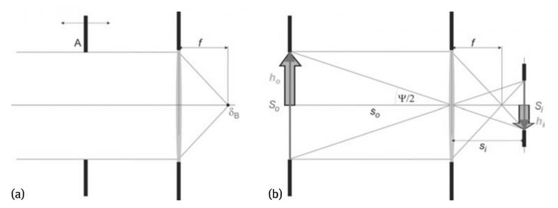
Fig.1 Illustration of (a) focusing and (b) imaging. In(a)the aperture A, which limits the beam diameter may be shifted as indicated by the arrow without affecting focusing (it may even be removed; this may be a somewhat simplified consideration). The dot indicated by δB is the focal spot F. Within aberration free geometrical optics it is a mathematical point which, of course, is infinitively small. However, within beam optics it has a finite size. In (b) the object may be the aperture around the solid arrow indicated with S0, or, e.g., provided by the open arrow (compare also to Figure 3)

The spot shows a light intensity distribution similar. The shape of the distribution depends on the beam shape in front of the optics. The diameter of the focal spot can be obtained from diffraction theory; see below equation δB

where
D is the beam diameter, respectively the width of the limiting aperture, for instance of a flat top profile in the near field.
κ is a constant that depends on the beam shape.

In addition it depends on the position within the profiles of the spot and the laser beam at which D and δ_B are respectively measured. a is a constant that describes the beam quality. It is a measure that describes wavefront distortions within the beam and also includes such ones that originate from aberrations from the optics. It should be noted that for Gaussian beams and perfect optics this is identical to the parameter “M²“.

Equation δ_B above can be derived by assuming a source at infinite distance that emits a spherical wave, thus being equivalent to the assumption of a plane wavefront that passes an aperture with a width D and afterwards an ideal lens. The aperture introduces an “intrinsic divergence”, which for instance yields to a first dark ring at the divergence angle θ₀.

Equation δ_B shows that, in particular, δ_B does depend on f/D. This ratio is the so-called f-number f# and is an important quantity in optics in general. It must be remarked that δ_B depends neither on f nor on D alone but only on the ratio of both. Furthermore it can be shown that the f-number, disregarding immersion optics, cannot be smaller than 0.5.

The goal of imaging is absolutely different. Images are taken to see what an object looks like. We would like to see its structures and hopefully also a lot of details. Thus the image should have a light distribution that is similar to that of the object, only the absolute size may differ. This is entirely different to focusing, where all of the light is concentrated within one spot and no structure information of an object is available at all. This is also obvious from SBN: for focusing N_SB =1 whereas imaging requires N_SB » 1. Focusing is closely related to Fraunhofer diffraction or far field, while imaging is governed by geometrical optics and near field. As an example, Figure 1b shows the image construction within geometric optics. The position of the image can be obtained by the thin lens equation

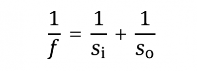
where S₀ and S_i are the object and the image distance, respectively.
It is obvious that the position of the image and that of the focal point are different. The size of the image S_i can be calculated form the object size S₀

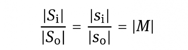
where M is the transversal or linear magnification of the imaging. It should be noted here that we disregard the direction of the distances and sizes and therefore use only the magnitude of these quantities. In a more rigorous consideration, which is done in subsequent chapters, the direction must be taken into account where a negative M accounts for an inverted image relative to the object, as can be seen in Figure 1.

In order to characterize images, some key parameters are required. Figure 2 illustrates the situation of imaging and shows the definitions used within this book. The object is imaged into the image plane, which in principle, extends laterally to infinity. Due to restrictions on the optical system, an image is restricted to a finite area.

Usually the optics is round and symmetric and thus, if it is well aligned, the image is restricted to the round area, termed image circle, as illustrated in the figure. The optical axis is perpendicular to the image and marks the center. If the sensor is centered as well, it cuts out a fraction of the image as shown by the rectangle in this figure. The width and the height of the sensor are designated by PW_sensor and PH_sensor, respectively. The sensor diagonal is d. The total height of the image of the scenery on the sensor is PH_sensor and lies within the image circle.

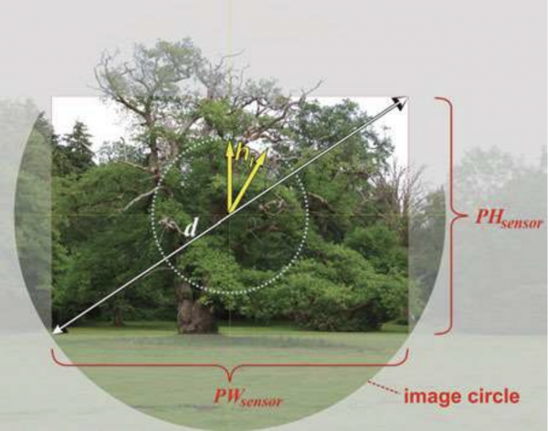
Fig. 2 Definitions of image parameters(see text)

Later on this image is reproduced as a printout, or displayed on a screen. The corresponding width and height will be termed PW and PH, respectively.

If we consider only a part of the original scenery as the object, for instance a branch of the displayed tree, its original size is given by S₀, its size in the image plane is S_i and the ratio of both quantities yields the transversal or linear magnification M. In many cases the term image height is used to describe the quality of the imaging process using rotationally symmetric optics. We then need to describe the transversal distance of an image point on the sensor from the optical axis. This distance is indicated in Figure 1 and Figure 2, respectively, by an arrow from the image center to any point and is designated by image height hi. Using this notation, for symmetry reasons, there is no directional dependence of h_i. The maximum value of h_i that is possible within the captured frame depends on direction (PH_sensor/2 ≤ h_i ≤ d/2).

For the generation of real images we need to discriminate three different conditions that result from the application of the thin lens equation and which are discussed for photography:

I) The object plane is nearly identical to the focal plane of the the lens, with S₀ ≈ f. Then a high magnification is achieved and the image plane is at a very large distance from the lens with S_i → ∞ and |M|» 1. This is the typical situation for microscopy where the optical system is not specified by its f-number f# and focal length but rather by its numerical aperture NA and magnification.

Ⅱ) The standard situation for photography and particularly for astrophotography is quite the opposite of microscopy.Here the object plane is at a large distance from the lens and particularly, S₀ is much larger than the focal length f of the system. As a consequence the image plane nearly coincides with the focal plane in the image space and the magnification becomes very small with |M|« 1.

Ⅲ) In the intermediate range for approximately 0.1 < |M|< 1 we have the situation of close-up photography or macro photography. For this type of imaging the image distance is significantly larger than the focal length of the lens which often requires special setups or lens constructions. Like for standard photography the optical system is rather described by its f-number and focal length.

This discrimination shows that the discussion about spatial optical resolution relates, for microscopy, to the object plane with the object being much smaller than the image whereas spatial resolution issues are more relevant in the image plane for photography. All spatial resolutions can also be expressed in terms of angular resolution. The angular resolution in the object space for distant objects, for instance as observed by astrophotography, is more meaningful than the spatial resolution in object space.

Here two remarks are very important:

Although formally (real) focusing maybe regarded as imaging of an object that is placed in infinity, and thus is demagnified to zero size with M → 0, such a consideration makes no sense at all; even if due to wave optics, the size remains finite. This is because the goal of imaging as an information transfer process is totally missed, due to the fact that one does not get any more information of the object’s structure. Again, focusing and imaging imply entirely different goals.

In photography people often talk of focusing: “before an image is captured, we have to focus”. However, of course, this is colloquial and not correct because as mentioned before, real focusing prevents any structural information and thus the goal of imaging. What people really mean is “rendering the image sharp” by fulfilling the lens Equation (thin lens equation) for a given object distance so with f given by the camera lens. However, because terms such as “one has to focus” or “focusing of the camera” are widespread, we also use this term if the meaning is unambiguous. Nevertheless we should be always aware of the real meaning of the terms!

Nevertheless, focusing and imaging are closely related by fundamentals of optics. In particular, if aberrations are mostly absent, the size of an “image point” δ, the resolution R within an image and the size of a focal spot δ_B, all obtained with the same optics, are not much different. The resolution may be obtained from Raleigh’s or Abbe’s criterion, respectively

where
NA is the numerical aperture.
K = 1.22 is valid for Raleigh’s criterion, whereas
K = 1 represents Abbe’s criterion.

From comparison of Equation δ_B to Equation R, it is obvious, that for κ =1.22 we get δ_B = 2·R.
Although the actual value of κ  is not of too much importance here, at least not for the discussion of the basics as in the present chapter, we may state, that for optical imaging, κ = 1.22 is mostly used and at least a good approximation.

According to this discussion, δ≈ δ_B, which then is given by Equation δ_B with κ = 1.22 and α = 1 for imaging with aberration free optics. Using this knowledge, the discrimination of imaging from focusing becomes even more clear. In particular, image quality is only good, if the number c of “image points” within the image is large. This is the case if PW, PH » δ or equivalently, if N_SB » 1 in a one-dimensional consideration. In two dimensions the result is straightforward. If NSB becomes smaller, the image quality becomes worse. The “worst image” and the largest “image point” size is PH (or PW; for simplicity in the following we assume PW = PH), neither the image size PH can become smaller than δ nor δ can become larger than PH. This is the situation of focusing and even the just used expression “worst image” should express the situation only formally. With respect to the above statement, we would like to state that talking about imaging requires at least a significant amount of “image points” within the image. There is no fixed limit; determining such a one is left to the “taste”of the reader.

Here we would like to add a further conclusive remark on that topic:
a) We talk about focusing when N_SB≈1.
b) We talk about imaging if N_SB » 1. This is the situation governed by geometrical optics although there might be severe corrections by wave optics.

Historically, in photography the size of an “image point” is given by the so-called circle of least confusion with a diameter of ui in the image plane. This is the limiting size of a spot that can still be perceived by the human eye. For normal viewing conditions we assume the angular resolution of the human eye as △φ_eye = 2′ of arc, which is equivalent to △φ_eye = 0.6 mrad. For high quality requirements the resolution of the eye is assumed to be of △φ_eye = 1′ of arc respectively △φ_eye = 0.3 mrad. As a consequence the maximum acceptable diameter ui for the circles of confusion, when viewing an image from the distance l, is given by:

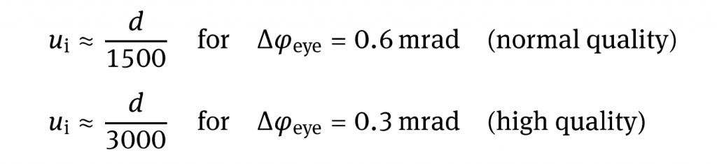
Due to the small value we have approximated tan (△φ_eye) by △φ_eye. Reproduced images such as typical rectangular image prints ale conventionally viewed at a distance that is approximately the same as their diagonal. The natural viewing angle is between 47° and 53° and the space bandwidth number of the eye is approximately N_SB,eye ≈1500 for normal quality resolution. This means that structures with a size of 1/1500 of the image diagonal d can still be perceived. For high quality requirements the resolution of the eye is assumed to be of △φ_eye = 1′ of arc respectively △φ_eye = 0.3 mrad and thus the allowable circle of confusion must be smaller or equal to 1/3000 of the diagonal. Thus we can define the acceptable diameter ui of the circle of confusion with respect to the image diagonal:

For an image print-out of 12 cm×18cm this means u_i ≈145μm for normal quality, and respectively, u_i ≈ 72 μm for high quality. As the image print-out is simply the magnification of the original image or a film or digital sensor, SBN remains unchanged， yielding a circle of confusion of about u_i ≈ 30μm for a full format sensor in normal quality and u_i ≈15 μm in high quality. If this print-out were a contact reproduction of a photographic film of the same format, the circle of confusion on the film would be identical to that of the image. As a consequence, if images are taken by cameras with different image sensors and then magnified to the same size, the requirements for acceptable circles of confusion are more demanding for smaller image sensors or films.

Thus lenses for mobile phone cameras require a much higher precision and quality than lenses for large format cameras. The relevance of the circle of confusion is discussed in the following chapters for different applications under different circumstances. The resolution of optical lenses is especially limited by lens aberrations and by the aperture stop of the lens. The resulting circle of confusion can be controlled by the f-number. Likewise the depth of field and depth of focus are controlled by the f-number and the acceptable circle of confusion.

It is important to note that the circle of confusion usually is defined for a larger value than δ_B, even in the case of small aberrations. The reason for this is that, e.g., a small value of “defocusing” is accepted, even for a high quality image. So far, we only considered the circle of confusion ui in the image plane. The associated value for the circle of confusion u0 in the object plane can be calculated by applying the image magnification, thus |u₀|= |u_i|/|M|. u₀ is a measure for the structure size in the object plane that is just at the limit of resolution by the optical system.