To get an introduction to imaging we may regard a very small object that we would like to image. Ideally this object should be a point, which means that it is infinitesimally small. In reality it is sufficient if it is very small, particularly if it is much smaller than the wavelength of light.

Now we do apply an optical instrument or system to get an image, which then is recorded by a two-dimensional detector and possibly stored by some additional device. For the moment we assume that the detector is an ideal one, which could detect the image with infinitesimally good quality. Of course, due to many reasons, this is not possible, but this does not play any role here. The recording device is not of interest in this article. The result of the imaging process is an “image point”, which always has a finite size and shows some intensity distribution. For the moment we must not make use of an exact definition of “intensity” as before, but it should be clear enough what we mean. Here we should mention that with “image point” we do not really mean an infinitesimally small point, but rather an extended spot. Only for simplicity and because it is widely used, in the following we will sometimes use the expression “image point” instead of “image spot”.

This distribution depends on the properties of the optical system and is not necessarily round or symmetric. Figure 1a shows an example of an image of a point object. We clearly see that it has some width δ, which could be measured at different positions within a line profile, such as δ_FWHM, which is measured at full width at half maximum (FWHM), etc. For the moment it is not of much importance which of the different values of δ we take, just that one is chosen.

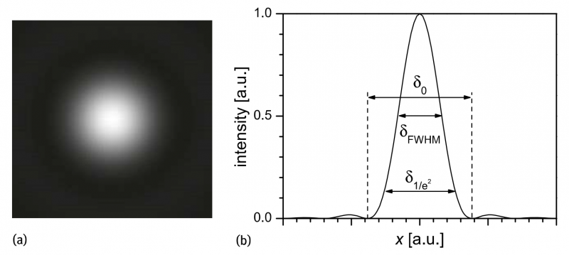
Fig.1: (a)Example of an image of a point object, ie., an“image point”. (b) Profile, e.g., measured along the horizontal or vertical line through the center or radial distribution of the light intensity, respectively. The arrows in (b) indicate the width of spot δ, measured at different positions, such as δFWHM measured at full width at half maximum (FWHM) or δ1/e2 measured at 1/e2 of the peak or δ0 measured between the indicated positions where the distribution becomes zero.

Now instead of taking just one simple object point we do take an extended macroscopic object that can be considered to be made of many of such object points. If, for simplicity we take each atom as one of those object points, of course, we do obtain a superposition of all corresponding “image points” and all corresponding” image point” light distributions.

This is the consequence of the linearity of Maxwell’s equations. Due to the huge amount of atoms within a macroscopic object, it is clear that this yields a tremendous amount of “image points” as well, and which becomes even infinite, if instead of atoms we consider infinitesimally small object points. From this we may conclude that absolutely every position within an image of a given size is the center of an “image point” and all “image point distributions” do overlap with other ones.

Although this seems to be a hopeless situation, it is not. Let us consider a simple model. First we have a look at two “image points” that are well separated (see Figure 2a). Here the distance d between them is much larger than their width δ and thus they could be well identified as two different points. If the distance becomes smaller and d ≈ δ then we are just at the resolution limit, i.e., we could just recognize that the two points are different ones (Figure 2c or Figure 2d).

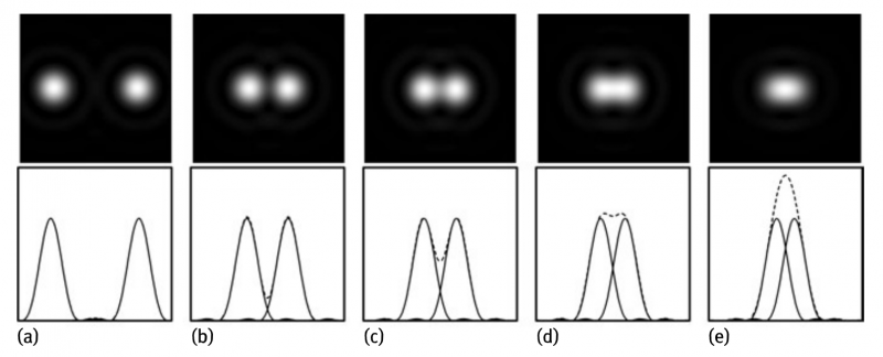
Fig. 2: Two image”points” located at different distances from each other. This is a demonstration of well resolved (a) and (b),just resolved (b) and(c) and hardly or not resolved dots (e), respectively. (d)corresponds to the Rayleigh criterion. The upper row shows the images, the lower one the profiles measured along the horizontal lines through the center of both points (solid lines:individual points, dashed lines and solid line in (a): superposition).

Here with resolution we mean the lateral optical resolution. For even smaller distances both points begin to merge to a single blur and could hardly be distinguished from each other (Figure 2c or Figure 2d or a situation where d is even smaller).We say those points are not resolved (Figure 2e).

Continuing our simple model, we will take a detector with a given size, say with a width PW in the horizontal direction and height PH in the vertical direction, respectively. But remember, apart from its finite size, it is still an ideal one which could display the image with infinitesimally good quality.

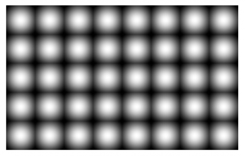
Fig.3: Simple model of an image made of selected “image points”

Then we begin to fill its plane with “image points”, however not with an infinite number of points. Instead, we start to put one“image point” somewhere (e.g., in the top left corner), and then we put the next neighbor in a horizontal direction at a distance, where we can resolve those two neighbored points. Then we continue this procedure in the horizontal direction and later on in the vertical direction as well, until the whole surface of the detector is filled (Figure 3).

Although there seems to be a straightforward similarity to newspaper pictures, which are made with a given finite number of real printer dots that are arranged in rows and columns and that may be identified as “image points” of that picture, it is very important to stress that the above discussion is related to a model that yields a finite number of selected “image points”. However, the physical image of any macroscopic object always still contains an infinite number of “image points”.

In case of a non ideal detector, the situation does not change in principle. Today usually such detectors are digital ones which are made of a two-dimensional array of photodiodes, which are named pixels, which means picture elements. If the pixel size is much smaller than δ, the situation is not much different from that with an ideal detector. If, on the other hand, δ is much smaller than the pixel size, then the pixels themselves take over the role of the imaging points.

Then, of course, the resolution is worse than δ. For the moment we may assume, that 1 pixel resembles one image point, but as we will see later, resolution is 2 pixels in 1D, or 4 pixels in 2D geometry, respectively. If the pixel size is the same as δ, we do have a complex situation where we do have to apply. However, also in such a case the basic idea of our simple model remains unchanged. The idea also remains unchanged, if we do take analogous detector such as a photographic film, where instead of regularily placed photodios, irregularily placed grains act as picture elements.

Furthermore, although the previous discussion is related to image observation or aquisition, it is applicable to the display of images as well. For instance, when a digital image is displayed on a digital screen, this screen is also made of pixels. In case of a monochrome display this is straightforward. In the case of color screens, each pixel is made of three subpixels that emit red, green and blue light, respectively. The three intensities are adjusted in a way that both the intended color and the total brightness of the pixel are reproduced correctly.

However, and although not subject of the present book, we would briefly like to comment that for physical prints generated with digital printers the situation is some-how more complex. For photographic papers the situation is different as well, but somehow similar to taking images on films. Again and similarly to before, one may describe the resolution of a print as the number of pixels per mm or the number of pixels per inch (ppi). But here the picture elements are made of printer dots.

Typically a matrix of 16×16 dots creates one pixel. Depending on the intended gray scale value of the pixel, this value is achieved by a mixture of dots within this matrix that together form the perceived gray scale. Then one observes the reflected light from the illuminated printed image as an average of the “black”and “white”dots with low and high reflectivity, respectively.

The observer should be so far away from the print that he only recognizes the matrix as one element with an average over the matrix elements. At best, the matrix is resolved as one element, but the individual dots are not resolved. This is similar to the averaging of the subpixels of a screen. For color prints, the final color of the pixel is also made of dots, but now with different colors. The background is not necessarily simple and is beyond the scope of the present work.

Altogether, the number of dots per mm or the number of dots per inch (dpi) is an important parameter for prints, and thus for the display of available images. But for the present book this is not an issue. We are concentrating on imaging itself. Discussion of displaying images is restricted to basic issues. In that sense, scanner-related topics are also not a subject under discussion, as scanning is different from imaging. There, lpi, i.e., lines per inch, is an important parameter